MultiImage Classification & ResNet 50 From Scratch

Introduction

In this notebook, we will learn how to classify images of Animals by developing ResNet 50 From Scratch

Load the images.

Visualize the Data distribution of all data.

Develop ResNet 50 From Scratch.

Train The Model.

Graph the training loss and validation loss.

Predict the results.

Confusion Matrix

Classification Report.

Prediction Comparison.

Install some of the Libraries

I have installed Split folders. I found this library very useful. You can split your data easily into the desired ratio and then can see it in the folder.

Importing Libraries

We are Importing Libraries.

Libraries which need for.

Image Processing.

Data visualization.

Making Model Architecture.

Setting Path

Now we are going to set the path of the data.

Importing Images

Import the Images

Now we going to make the data frame of the image data so we can do some anylasis on the data.

you will get output like this.

Now count the total number of images of each class.

you would get output like this.

Total Data Distribution

Now let’s visualize the data so we can have a better understanding

we will use the Plotly library to make Bar charts and Pie chart

A barchart will be some thing like this

Siplting the Data into Train test and Val

setting Path

calculate the total amount of images in each sub-data set.

The out put will be

lets explore the Train Data set.

First, make the data frame of the train data set.

Second count the number of Images of each class

You can visualize the data in form of a Bar and chart by repeating the process that we done previously.

Displaying The Images

You will get output like this.

The data analysis part has been done. we just completed our first module of the project

Now Prepare the data set for the model.

Image Data Generator

output

You can see it automatically detected the number of the classes

ResNet50

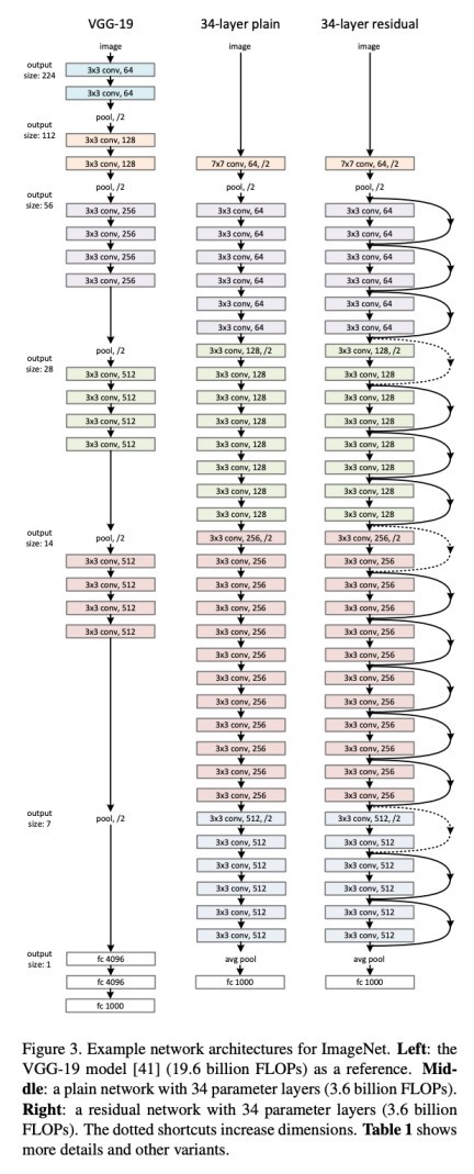
It is very important to understand the ResNet. The advancement in the computer vision task was due to the breakthrough achievement of the ResNet architecture.

The architecture allows you to go deeper into the layers which are 150+ layers.

It is an innovative neural network that was first introduced by Kaiming He, Xiangyu Zhang, Shaoqing Ren, and Jian Sun in their 2015 computer vision research paper titled ‘Deep Residual Learning for Image Recognition.

More Details about the paper can be found here Deep Residual Learning for Image Recognition

Before Resnet, In theory, the more you have layers the loss value reduces and accuracy increases, but in practically that did not happen. The more you have layers the accuracy was decreasing.

Convolutional Neural Network has the Problem of the “Vanishing Gradient Problem” During the Backpropagation the value of gradient descent decreases and there are hardly any changes in the weights. To overcome this problem Resnet Comes with Skip Connections.

Skip Connection — Adding the original input to the output of the convolutional block.

Basically, resnet has two parts One is an Identity block and the other one is a convolutional block.

7.1 Identity Block

The value of ‘x’ is added to the output layer if and only if the.

Input Size == Output Size.

Convolutional Block

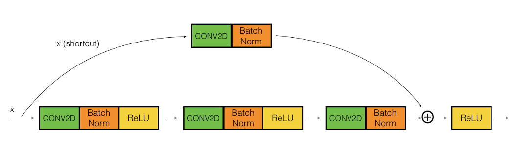
if Input Size != Output Size.

we add a ‘convolutional block’ in the shortcut path to make the input size equal to the output size.

let’s combine the identity and convolutional block

In the last line “headModel = Dense( 10,activation=’softmax’, name=’fc3',kernel_initializer=glorot_uniform(seed=0))(headModel)”

you can change the number of classes according to your data set as well by changing the 10 to your number of classes , suppose you have 5 classes then the line would be (headModel = Dense( 5,activation=’softmax’, name=’fc3',kernel_initializer=glorot_uniform(seed=0))(headModel))

From here there are two ways, Either you can load the weitghs and use the pre-trained weights for the classification or you train your model from the scratch.

For Training from scratch, you just compile the model and then train that model.

Pre-Trained Weights.

Train the model

A callback is an object that can perform actions at various stages of training (e.g. at the start or end of an epoch, before or after a single batch, etc).

Early Stopping is used to prevent the model from overfitting.

Train command

Model Evaluation

Classification Report

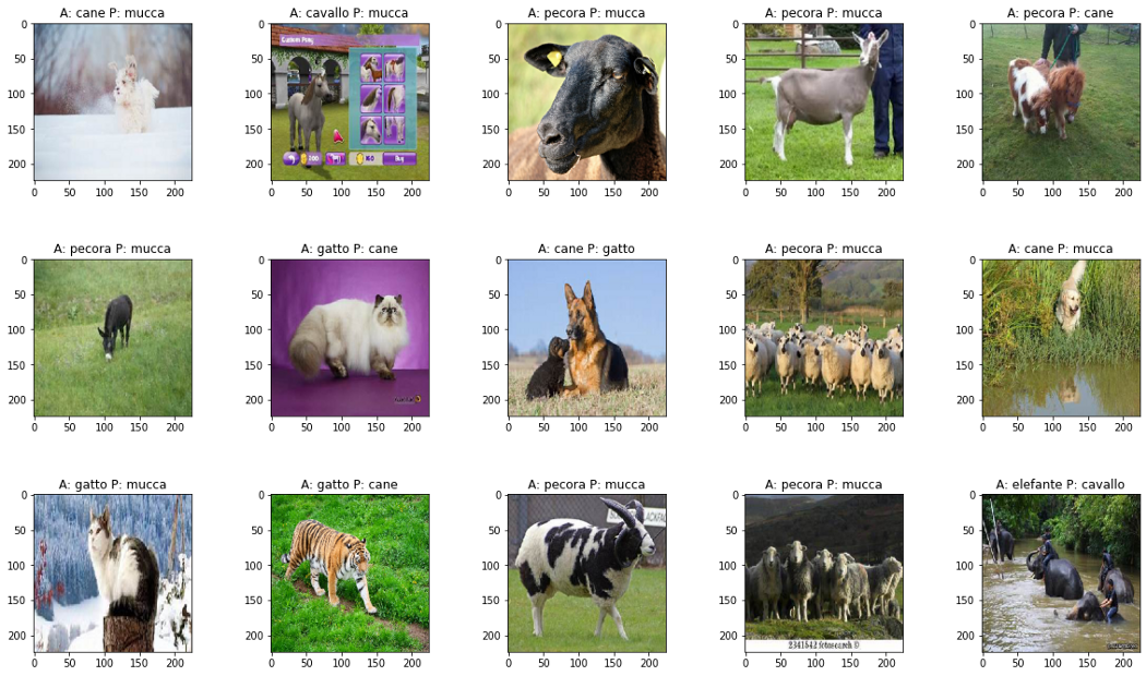
Prediction Comparison

Making Data Frame of the Prediction

You will get this output

For loading Images

Correctly classified.

Misclassified.

For detailed working code, you can go to this link and then copy and edit the code fromKaggle

Please hit the clap button Your little appreciation will boost my motivation 🙏🙏

GitHub Repo

https://github.com/106AbdulBasit/ResNet50-Weights

Don’t Forget to Vote up if you like my work