Facial Emotions Recognition through Deep learning

We will create a real-time facial emotions recognition system using python. This system can be tested on both videos including webcam and photos.

In this project, we will create a real-time facial emotions recognition system using python. This system can be tested on both videos including webcam and photos.

Here’s a demo video of the project before we dive into the code:

Dataset

FER2013 dataset was used for this project. FER2013 is an open-source facial emotions recognition dataset containing approximately 30,000 grayscale, resized images 48×48 pixel images. The goal is to put each face into one of seven categories (0=Angry, 1=Disgust, 2=Fear, 3=Happy, 4=Sad, 5=Surprise, 6=Neutral) depending on the emotion expressed in the facial expression. There are 28,709 instances in the training set and 3,589 examples in the public test set.

Import Libraries and Dependencies

Tensorflow library was used for training the machine learning model along with Keras for developing a neural network architecture.

                import numpy as np 
import pandas as pd 
import os 
import tensorflow as tf 
from tensorflow import keras 
from keras.models import Sequential 
from keras.preprocessing.image import ImageDataGenerator, load_img from keras.layers import Conv2D, Dense, BatchNormalization, Activation, Dropout, MaxPooling2D, Flatten 
from keras import optimizers from tensorflow.keras.optimizers import Adam, RMSprop, SGD 
from keras.callbacks import ModelCheckpoint,EarlyStopping 
import datetime from keras import regularizers 
import matplotlib.pyplot as plt from keras.utils.vis_utils 
import plot_model from keras.callbacks import ReduceLROnPlateau

Loading the dataset

For this project, the training was performed in Google Colab. Hence the training and testing dataset were unzipped in the colab.

Mounting Google Drive:

                from google.colab import drive drive.mount('/content/gdrive')

Installing unrar so that it can be used to retrieve data. Note that you need to keep the zipped folders of dataset in your drive

                !pip install unrar !unrar x gdrive/My\ Drive/FER-7-CNN/FERtrain.rar !unrar x gdrive/My\ Drive/FER-7-CNN/FERtest.rar

Exploring Dataset

                train_dir = "/content/FERtrain/"
test_dir ="/content/FERtest/"
row , col = 48 , 48
classes = 7
def count_exp(path, set_):
dict_ = {}
for expression in os.listdir(path):
dir_ = path + expression
dict_[expression] = len(os.listdir(dir_))
df = pd.DataFrame(dict_, index=[set_])
return df
train_count = count_exp(train_dir, 'train')
test_count = count_exp(test_dir, 'test')
print(train_count)
print(test_count)

                train_count.transpose().plot(kind='bar')

                test_count.transpose().plot(kind='bar')

                plt.figure(figsize=(14,22))
i = 1
for expression in os.listdir(train_dir):
img = load_img((train_dir + expression +'/'+ os.listdir(train_dir + expression)[5]))
plt.subplot(1,8,i)
plt.imshow(img)
plt.title(expression)
plt.axis('off')
i += 1
plt.show()

Preparing Dataset for Training

                train_datagen = ImageDataGenerator(rescale=1./255,
horizontal_flip=True,
validation_split=0.2)
training_set = train_datagen.flow_from_directory(train_dir,
batch_size=64,
target_size=(48,48),
shuffle=True,
color_mode='grayscale',
class_mode='categorical',
subset='training')
validation_set = train_datagen.flow_from_directory(train_dir,
batch_size=64,
target_size=(48,48),
shuffle=True,
color_mode='grayscale',
class_mode='categorical',
subset='validation')
test_datagen = ImageDataGenerator(rescale=1./255,
horizontal_flip=True)
test_set = test_datagen.flow_from_directory(test_dir,
batch_size=64,
target_size=(48,48),
shuffle=True,
color_mode='grayscale',
class_mode='categorical')
Output: Found 22968 images belonging to 7 classes. Found 5741 images belonging to 7 classes. Found 7178 images belonging to 7 classes.
#labels 
training_set.class_indices
Output:
{'angry': 0, 'disgust': 1, 'fear': 2, 'happy': 3, 'neutral': 4, 'sad': 5, 'surprise': 6}

Model Architecture

                weight_decay = 1e-4
num_classes = 7
model = tf.keras.models.Sequential()
model.add(Conv2D(64, (3,3), padding='same', kernel_regularizer=regularizers.l2(weight_decay), input_shape=(48,48,1)))
model.add(Activation('relu'))
model.add(BatchNormalization())
model.add(Conv2D(64, (3,3), padding='same', kernel_regularizer=regularizers.l2(weight_decay)))
model.add(Activation('relu'))
model.add(BatchNormalization())
model.add(MaxPooling2D(pool_size=(2,2)))
model.add(Conv2D(128, (4,4), padding='same', kernel_regularizer=regularizers.l2(weight_decay)))
model.add(Activation('relu'))
model.add(BatchNormalization())
model.add(Conv2D(128, (4,4), padding='same', kernel_regularizer=regularizers.l2(weight_decay)))
model.add(Activation('relu'))
model.add(BatchNormalization())
model.add(MaxPooling2D(pool_size=(2,2)))
model.add(Dropout(0.2))
model.add(Conv2D(256, (4,4), padding='same', kernel_regularizer=regularizers.l2(weight_decay)))
model.add(Activation('relu'))
model.add(BatchNormalization())
model.add(Conv2D(256, (4,4), padding='same', kernel_regularizer=regularizers.l2(weight_decay)))
model.add(Activation('relu'))
model.add(BatchNormalization())
model.add(MaxPooling2D(pool_size=(2,2)))
model.add(Dropout(0.25))
model.add(Conv2D(512, (3,3), padding='same', kernel_regularizer=regularizers.l2(weight_decay)))
model.add(Activation('relu'))
model.add(BatchNormalization())
model.add(Conv2D(512, (3,3), padding='same', kernel_regularizer=regularizers.l2(weight_decay)))
model.add(Activation('relu'))
model.add(BatchNormalization())
model.add(MaxPooling2D(pool_size=(2,2)))
model.add(Dropout(0.3))
model.add(Flatten())
model.add(Dense(256, activation="linear"))
model.add(BatchNormalization())
model.add(Activation('relu'))
model.add(Dropout(0.45))
model.add(Dense(256, activation="linear"))
model.add(BatchNormalization())
model.add(Activation('relu'))
model.add(Dropout(0.45))
model.add(Dense(num_classes, activation='softmax'))
model.compile(loss='categorical_crossentropy', optimizer = Adam(0.0001) , metrics=['accuracy'])
model.summary()

Model Training

                checkpointer = [EarlyStopping(monitor = 'val_accuracy', verbose = 1, restore_best_weights=True,mode="max",patience = 5),
ModelCheckpoint(
filepath='model.weights.best.hdf5',
monitor="val_accuracy",
verbose=1,
save_best_only=True,
mode="max")
]
checkpointer = [EarlyStopping(monitor = 'val_accuracy', verbose = 1, restore_best_weights=True,mode="max",patience = 5),
ModelCheckpoint(
filepath='model.weights.best.hdf5',
monitor="val_accuracy",
verbose=1,
save_best_only=True,
mode="max")
]
steps_per_epoch = training_set.n // training_set.batch_size
validation_steps = validation_set.n // validation_set.batch_size
history = model.fit(x=training_set,
validation_data=validation_set,
epochs=40,
callbacks=[checkpointer],
steps_per_epoch=steps_per_epoch,
validation_steps=validation_steps)

Evaluating Model Performance

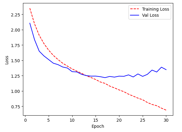
PLOTTING TRAINING LOSS/ VAL-LOSS VS EPOCHS

                training_loss = history.history['loss']
val_loss = history.history['val_loss']
plt.rcParams['figure.figsize'] = [10, 5]
plt.style.use(['default'])
# Create count of the number of epochs
epoch_count = range(1, len(training_loss) + 1)
# Visualize loss history
plt.plot(epoch_count, training_loss, 'r--')
plt.plot(epoch_count, val_loss, 'b-')
plt.legend(['Training Loss', 'Val Loss'])
plt.xlabel('Epoch')
plt.ylabel('Loss')
plt.show()

PLOTTING ACCURACY/VAL_ACCURACY VS EPOCHS

                training_accuracy = history.history['accuracy']
val_accuracy = history.history['val_accuracy']
# Create count of the number of epochs
epoch_count = range(1, len(training_accuracy) + 1)
# Visualize loss history
plt.plot(epoch_count, training_accuracy, 'r--')
plt.plot(epoch_count, val_accuracy, 'b-')
plt.legend(['Training Accuracy', 'Val Accuracy'])
plt.xlabel('Epoch')
plt.ylabel('Accuracy')
plt.ylim(top = 1)
plt.show()

Saving Model

Saving the trained model is important so that it can be loaded later for testing without the need of training all over again

                model.save("fer7_model.h5")

Test dataset accuracy

                print(f"Test accuracy = {model.evaluate(test_set ,batch_size=test_set.batch_size,steps=test_set.n // test_set.batch_size)[1]*100}%") 

Output:
112/112 [==============================] - 3s 22ms/step - loss: 1.2351 - accuracy: 0.6274 Test accuracy = 62.73716688156128%

Plotting predictions

                # next function assigns one batch to variables, i.e x_test,y_test will have 64 images
x_test,y_test = next(test_set)
predict = model.predict(x_test)
class_labels = test_set.class_indices
class_labels = {v:k for k,v in class_labels.items()}
figure = plt.figure(figsize=(20, 8))
for i, index in enumerate(np.random.choice(x_test.shape[0], size=24, replace=False)):
ax = figure.add_subplot(4, 6, i + 1, xticks=[], yticks=[])
ax.imshow(np.squeeze(x_test[index]))
predict_index = class_labels[(np.argmax(predict[index]))]
true_index = class_labels[(np.argmax(y_test[index]))]
ax.set_title("{} ({})".format((predict_index),
(true_index)),
color=("green" if predict_index == true_index else "red"))

Real time Testing (Webcam/Videos)

Testing part is executed on Jupyter Notebook and not on Google Colab. Make sure to provide the path for trained model which we saved after the training. Drawing a rectangle over the face is an optional part. To run that part make sure you provide the path of frontal face haarcascade xml file

                import os
import cv2
import numpy as np
from tensorflow.keras.preprocessing import image
import warnings
warnings.filterwarnings("ignore")
from tensorflow.keras.preprocessing.image import load_img, img_to_array 
from tensorflow.keras.models import  load_model
import matplotlib.pyplot as plt
import numpy as np
# load model
model = load_model("FER_7/fer7_model.h5")
face_haar_cascade = cv2.CascadeClassifier(cv2.data.haarcascades + 'haarcascade_frontalface_default.xml')
#Optional part for writing video
video_cod = cv2.VideoWriter_fourcc(*'XVID')
video_output= cv2.VideoWriter('out.mp4',
                      video_cod,
                      10,
                      (1000, 700))
cap = cv2.VideoCapture(0)
while True:
    ret, test_img = cap.read()  # captures frame and returns boolean value and captured image
    if not ret:
        continue
    gray_img = cv2.cvtColor(test_img, cv2.COLOR_BGR2GRAY)
faces_detected = face_haar_cascade.detectMultiScale(gray_img, 1.32, 5)
for (x, y, w, h) in faces_detected:
        cv2.rectangle(test_img, (x, y), (x + w, y + h), (255, 0, 0), thickness=7)
        roi_gray = gray_img[y:y + w, x:x + h]  # cropping region of interest i.e. face area from  image
        roi_gray = cv2.resize(roi_gray, (48, 48))
        img_pixels = image.img_to_array(roi_gray)
        img_pixels = np.expand_dims(img_pixels, axis=0)
        img_pixels /= 255
predictions = model.predict(img_pixels)
# find max indexed array
        max_index = np.argmax(predictions[0])
emotions = ["Angry", "Disgust", "Fear", "Happy", "Neutral", "Sad", "Surprise" ]
        predicted_emotion = emotions[max_index]
        cv2.putText(test_img, predicted_emotion, (int(x), int(y)), cv2.FONT_HERSHEY_SIMPLEX, 1, (0, 0, 255), 2)
resized_img = cv2.resize(test_img, (1000, 700))
    cv2.imshow('Facial emotion analysis ', resized_img)
    
    #optional
    video_output.write(resized_img)
if cv2.waitKey(25) & 0xFF == ord('q'):
      break
cap.release()
#optional
video_output.release()
cv2.destroyAllWindows

Originally published at https://visione.website on June 9, 2022.