Data Structures And Algorithms: Big O Notation

The above function iterates through the sample_array a certain number of times, the size of the array is unknown to us at this point.

So we also want to know how much time does it take to run the above function, independent on various factors such as the processing power of the computer, the operating system, programming language, etc.

Let’s rather ask this question; “how does the runtime of the function grow as the size of the input grows”?

Well the more elements there are in a given array, the more elements there are to add up.

The question we just asked is answered by The Big O Notation and Time Complexity.

Big O notation is an industry standard for measuring efficiency and performance of your program based on four criteria:

• The ability to access a specific element within a data structure
• Searching for a particular element within a data structure
• Inserting an element into a data structure
• Removing an element from a data structure

Let’s say we need to store data which performs good at accessing elements quickly or a data structure that can add or delete elements easily, which do we use? Well we have the mathematical tool Big O notation to help us decide.

These four criteria accessing, searching, inserting and deleting are all sorted using Big O notation time complexity equations.

This works by inserting the size of the dataset as an integer n and in return we get the number of operations that need to be conducted by the computer before the function can finish.

The integer n represents the size of the data set/ the amount of elements contained within the data structure.

So if we have an array with size of 100 then n would be equal to 100, n=100.

We would place 100 into the different efficiency equations and returned to us would be the number of operations needed to be completed by the computer.

Determining The Time Complexity

Time complexity is a method used to show how the runtime of a function increases as the size of the input(n) increases.

How do we determine time complexity? Well we have two rules we use:

1. Keep the fastest Growing Term
2. Drop constants

Example:

Time = a*n+b

Let’s start with the first rule, we keep the fastest growing term which is a*n, b is our constant and thus we drop it.

Now we have Time = a*n and we implement our second rule stating that we must drop all constants, we are just left with one, which is a.

When we drop a we are left with Time = n, also referred to as Big O(n).

Big O Notation Time Complexity Types

There are six most common types of time complexity equations namely;

• O(1), O(n), O(logn), O(nlogn), O(n^2), O(2^n)

These vary from most efficient to least efficient, in this article we will only be discussing three of the six.

O(1)

The best a data structure can perform on each criteria is O(1), regardless of your data set the task will be completed in a single instruction.

If our data set has 50 elements, the computer will finish the task in one instruction, same applies if our data set has 1billion elements the computer will still complete the task in one instruction, it does not matter.

O(1) is the gold standard, the Beyoncé of Big O notation when it comes to time complexity equations.

Above we have a function that has an array of 5 elements, and we will name it example_function, it accepts given_array as an input.

So we define a variable total and set it to 0, then return total.

O(logn)

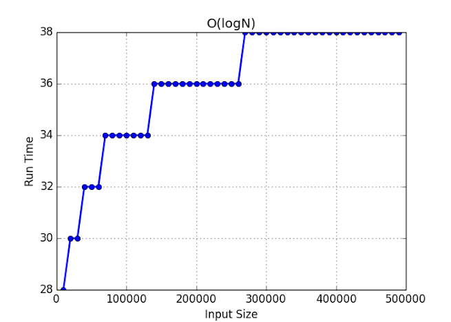
The next fastest type of time complexity equation is O(logn) which gets more efficient as the size of the dataset increases, the value of data vs time graph follows a logarithmic curve, the larger the dataset used the more beneficial it is.

O(n)

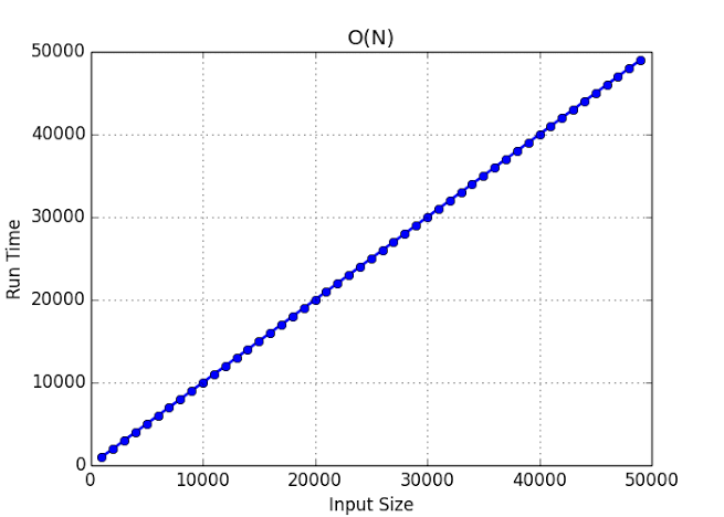
This is the last of the decent equations, with a linear graphical representation, the number of elements you add to a dataset and the amount of instructions needed to complete the function are equal.

To perform a function with a time complexity of O(n) on a dataset with 1 million elements then 1 million instructions are needed.

Lets we have a function which takes an array (given_array) as input and finds the sum within the array.

As the size grows the time also grows thus this is a linear function, the time it takes to run this program is linearly proportional to the array size.

Any linear function can be represented as:

Time = a*n +b

Let’s calculate how we got to O(n):

Time = a*n +b, the first rule is we are going to keep the fastest growing term, b is the constant and we drop it. The fastest growing term is a*b, let’s say n is 300 and a is 2 we will have 600.

The second rule is that we drop any constant:

Time = a*n, our constant here is a and when we drop it we are left with n.

We are left with time = O(n)